The Metascape forum receives many questions about how enrichment bar graphs and heatmaps are created. This blog post explains the backend algorithms.
For a given gene list, we use the accumulative hypergeometric test (or Fisher’s exact test) to compute the p-values and enrichment factors for each ontology category (referred to as a GO term or simply a term hereafter). The detailed statistics behind enrichment analysis were described previously [here]. We explained in the Metascape paper [1] that “ontology terms found in GO form a hierarchical structure of increasing granularity, making the terms inherently redundant. Terms across different ontology sources, such as GO, KEGG, and MSigDB, etc. can be closely related as well. As a result, functional enrichment analysis can identify overlapping or related terms, making it difficult to extract non-redundant and representative processes to report in the analysis output.”
Representative Terms
We cluster all enriched terms into groups and select one term from each group as the representative. For instance, the enriched terms are grouped as \(\{T_{11}^*, T_{12}, T_{13}\}\), \(\{T_{21}^*, T_{22}, T_{23}, T_{24}\}\), \(\{T_{31}^{*}, T_{32}\}, \dots\)
The first group contains three terms \(T_{11}\), \(T_{12}\), and \(T_{13}\). The group members are sorted by their p-values, where \(T_{11}\) has the smallest p-value (most negative \(\log P\)). Terms \(T_{11}\), \(T_{21}\), and \(T_{31}\) have an asterisk superscript to indicate that they are considered the best representatives of their respective groups. These asterisk terms are displayed in the bar graph and heatmap. The bar graph and heatmap contain the top 20 groups, but the plots for the top 100 groups are also available in the zip file. Results for all enriched terms are still available in the file named “Enrichment_GO/_FINAL_GO.csv” as part of the zip pakcage. This explains why term \(T_{12}\) is not found in the plots, as \(T_{11}\) is its proxy. The results for \(T_{12}\) is considered redundant to those of \(T_{11}\) , but nevertheless \(T_{12}\) can be found in “_FINAL_GO.csv”.
Excel Sheet “Enrichment”
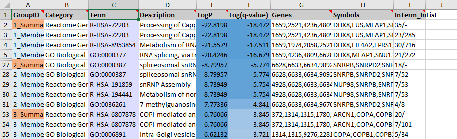
The enrichment results for the top 20 groups are also reported under the “Enrichment” sheet of the “metascape_result.xlsx” file. The top three groups are shown in the screenshot (Figure 1). The first group contains 24 members (Row 3-26, where Row 6-26 are hidden). Row 3 is the representative term for the first group, with the lowest \(Log P\) value of -22.8198 corresponding to 23 (#GeneInGOAndHitList) out of the 285 (#GeneInGO) genes. This representative entry is cloned into Row 2. Row 2 summarizes the whole group (highlighted in orange). We can see that Row 2 basically shows the same information as Row 3, except “Genes” and “Symbols” are the combination of all “Genes” and “Symbols” from Row 3 to Row 26. There are a total of 35 (#GeneInGOAndHitList) genes, therefore, we show “35” in column I. Since the summary row does not map into one specific term, there is no (#GeneInGO) count (shown as a dash in Row 2 and Column I).
Clustering Algorithm
Each enriched term contains a list of genes (refer to column G in Figure 1). If we take all enriched terms as columns and all genes (from all terms) as rows, we have a binary membership matrix (Figure 2.a). We can then compute the similarity score between a pair of terms based on Kappa statistics. Some details were described by DAVID [2] and reproduced in this blog for readers’ convenience.
Figure 2.a shows an example of 7 total genes and 7 total terms. Term \(T_{i}\) has 3 genes and \(T_{j}\) has 4 genes. \(T_{i}\) and \(T_{j}\) have 6 out of 7 rows in common (3 ones and 3 zeros, \(G_{q}\) is not shared). By random chance, the probability of \(T_{i}\) and \(T_{j}\) both having the membership 1 for a given gene is \(\frac{3}{7} \times \frac{4}{7}\) and they both having membership value 0 for a given gene is \(\frac{4}{7} \times \frac{3}{7}\) . Therefore, the probability of \(T_{i}\) and \(T_{i}\) sharing the same membership value is the sum of the two, i.e., \(\frac{24}{49}\). We know that at most \(T_{i}\) and \(T_{j}\) share 100% of the rows, so we define the \(\kappa\) score as:
\[\kappa = \frac{\frac{6}{7} – \frac{24}{49}}{1- \frac{24}{49}} = 0.72,\]
where the denominator is simply a normalization factor equal to the largest possible value the numerate can take. The \(\kappa\) similarity score will be a value maxed at \(1\) if two terms are identical, \(0\) if two terms are no more similar than random, and negative if two terms are even less similar compared to random. The distance between two terms is defined as \(1-\kappa\). After we compute \(\kappa\) for all pairs of terms, we can use the similarity matrix (or distance matrix) to cluster terms. DAVID invented an ad hoc fuzzy cluster algorithm [3], which we consider unnecessary. We simply run the standard hierarchical clustering algorithm with average linkage as described below.
In Figure 2.b, the hierarchical clustering algorithm first links two terms that are most similar (the smallest distance), so \(c\) and \(d\) are linked together first into tree \((c, d)\). Then \(a\) and \(b\) are linked into tree \((a, b)\), followed by tree \((e, f)\). The \((a, b)\) tree and \((c, d)\) tree are linked next, where the distance of the two subtrees is defined as:
\[d_{(a,b),(c,d)}=\frac{1}{4}(d_{a,c}+d_{a,d}+d_{b,c}+d_{b,d})\]
Finally, tree \((a, b, c, d)\) is constructed, then a larger tree connect \((a, b, c, d)\) and \((e,f)\).
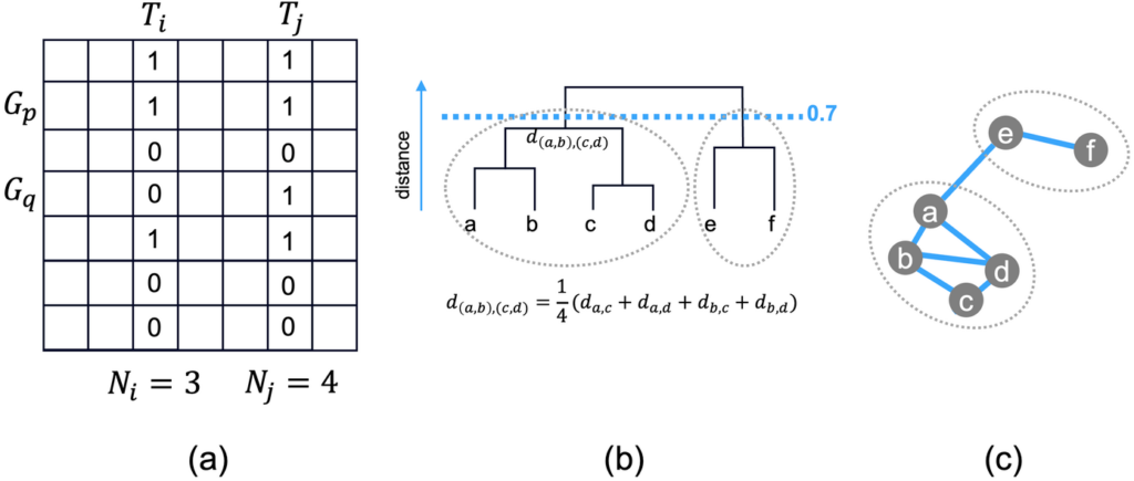
We apply a distance cutoff of 0.7 (\(\kappa\) similarity 0.3), shown as the blue dashed line (Figure 2.b). Each subtree below the cutoff forms a group (or cluster). Therefore, \((a, b, c, d)\) form one group, and \((e, f)\) forms another group.
Due to the way distances are defined, even if \((a, b)\) and \((c, d)\) form a final group with a distance less than 0.7, it does not mean that all pairwise members have a distance below 0.7. Some distances can be higher, as long as the average is below 0.7. Assume term \(b\) has the lowest \(\log P\) among \((a, b, c, d)\); \(b\) will become the representative term for this group.
Network Visualization
Bar graphs and heatmaps only show the representative terms; otherwise, the visualization will be too busy to be useful for visual interpretation. To visualize non-representative terms, we can use a network visualization (Figure 2.c).
We show the 6 genes as nodes of a network. When a pair of nodes has a similarity \(\kappa\) higher than 0.3, they are connected by a blue edge. We see that \((a, b, c, d)\) and \((e, f)\) are grouped together respectively. However, there is no blue edge linking \(a\) and \(c\), implying \(d_{a,c} > 0.7\). Nevertheless, \(a\) and \(c\) still belong to the same group, as \((a, b)\) and \((c, d)\) have an average similarity above 0.3. Similarly, there is an edge connecting \(a\) and \(e\), even though they belong to two groups.
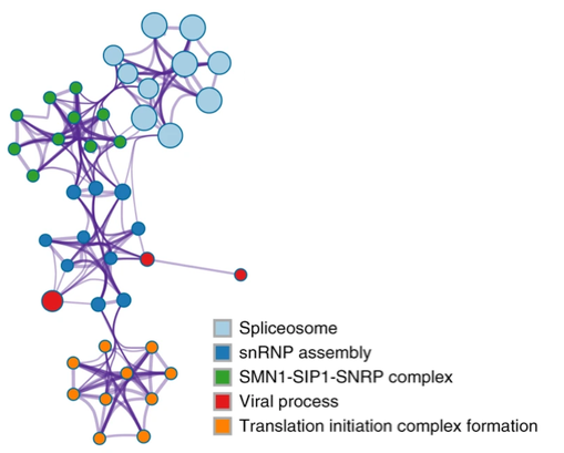
In the example network below (extracted from [4]), we see five groups consisting of densely connected members. If a group contains many members, we display at most top 10 members to keep the visualization interpretable. There are a few edges linking different clusters, indicating they are distant but related biological processes. We see that spliceosome processes are closely related to SMN1 complex, which in turn is related to snRNP assembly, which is further connected with viral processes and translation initiation complexes. To visualize individual nodes, open the “Enrichment_GO\GONetwork.cys” session file in Cytoscape.
Reference
- https://www.nature.com/articles/s41467-019-09234-6
- https://david.ncifcrf.gov/helps/linear_search.html#kappa
- https://david.ncifcrf.gov/helps/functional_classification.html#heuristic
- https://www.nature.com/articles/s41467-019-09234-6/figures/2